Build a swept volume for a turned part

Preface

Lathe machines are commonly used for manufacturing because of their relatively low cost and inherent simplicity of the process. At the same time, lathes are often combined with milling that serves as a post-process for finishing up a turned workpiece with non-rotational features.

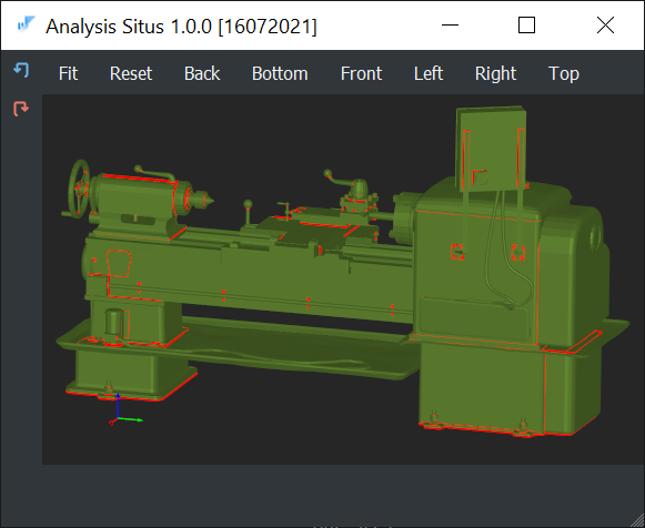1K62.

There are several questions you might want to ask looking at a turned part at hand:

• How much of it can be manufactured on a lathe machine? Well, to be cost-efficient, the more the better.
• What is the envelope swept by this turned piece when rotating? That is something you might need for collision checks, e.g. in milling simulation.

This article aims at describing the computational principles one might want to follow to build up a swept volume of a rotary part (that's a special case of a swept volume problem). You only need to know the axis of rotation, which might be the lathe axis or a spindle axis for a milling tool. The purpose of the algorithm is to build the minimal solid of revolution containing the original part. This solid is sometimes named a Maximum Turnable State (MTS) of the geometry [Yip-Hoi, D., & Dutta, D. (1997). Finding the maximum turnable state for Mill/Turn parts. CAD Computer Aided Design, 29(12), 879–894.]. From a lathing standpoint, MTS represents an intermediate state of the workpiece geometry from which no more material can be removed by turning. The result of a Boolean subtraction between a stock shape and the MTS gives what's called the Maximum Turnable Volume (MTV).

Simple & stupid

The MTS is a solid of revolution and that kind of a solid is obtained by sweeping a generatrix curve around an axis. Therefore, if we want to build MTS, it's sufficient to extract the generatrix curve. Although there are some attempts to generate MTS based on the recognized turned features of a model, I wouldn't go for such methods unless I really have to. The reason for that is the ultimate complexity of the approach we end up with. If five years spent on feature recognition taught me something, it's that feature recognition is far never perfect to rely upon. Whenever I can do the job in a simple and stupid way, I would prefer doing so and not overcomplicate the thing.

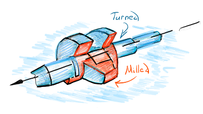Turned/milled part the best I could draw one.

One simple approach was reported by M. Watkins et al [Watkins, M., Rahmani, K., & D’Souza, R. (2008). Finding the maximal turning state of an arbitrary mesh. 2007 Proceedings of the ASME International Design Engineering Technical Conferences and Computers and Information in Engineering Conference.]. They sample the rotation axis (presumably OX) with the even distribution of slices and then find the intersection points between the slice planes and mesh edges. Since the slices are all sorted, the extreme values of the intersection points are sorted as well. It's trivial then to construct the profile curve. Well, this really sounds simple and stupid, so let's give it a try.

Mesh data structure

One should carefully choose the mesh data structure. The good choice will pay off, while an unsuitable data structure will make you constantly working things around instead of focusing on the problem. And you know what? There seems to be no such data structure that would serve all the cases equally well. While worked at OCC, I was somehow blindly assured that everything should be based on Poly_Triangulation, which is the simplistic mesh representation for facets distributed by B-rep faces. Then, OCC came up with another data structure (Poly_CoherentTriangulation) that offers a more editable and iteratable mesh, although it's not a part of the OpenCascade data model anymore. Something could also be grabbed from Salome if you manage to find where it's all hosted.

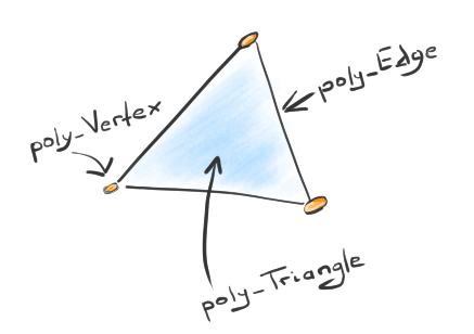The elements of a mesh data structure.

It took time and it required a certain shift in my mindset to realize that the data structures should always be chosen application-wise. There's no such a thing as a "good" data structure. There could only be a data structure good enough for a specific problem. That's actually a trivial foolish discovery if you think about it, but the implications are severe. In practice, it means that instead of componentizing yet another "now perfect" data structure (look at OpenMesh as an example), it might be better to copy & paste your stuff for exclusive use in your target algorithm. For example, a decimation algorithm might require a half-edge data structure. Working with dirty scans might demand a somewhat less restrictive data structure that perhaps allows for non-manifold triangles. Who said that copying & pasting code is a bad thing? I call bullshit on that.

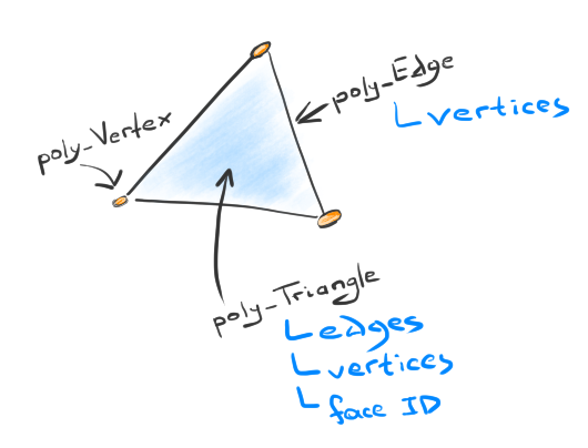The elements of a mesh data structure with references.

Then, there's also a question of relationships between your mesh data structure and the CAD geometry. Are they divorced? Do you have a reference mechanism to attribute a single facet as belonging to a certain CAD face? And there're many questions like that. Long story short, for the MTS algorithm, I use a variation of poly_Mesh hand-made data structure. It's not ideal by any means, but there's one killing feature of this in-house data structure: I can do whatever I want with it and disregard any product boundaries because there are no boundaries to respect. I simply don't care about the architecture of any 3-rd party product. No product no pain. Free love.

Watkins algorithm

The algorithm assumes that the axis of revolution is aligned with the global OX axis. Such an assumption does not take away the generality of the approach as you can always reorient your part to satisfy that requirement. All in all, the implementation of M. Watkins' algorithm is pretty straightforward as all you need is to find the intersection points of all mesh edges with the slicing planes. I'm not sure it's written in the original paper, but you also have to check that the intersection points fall inside the corresponding edges to avoid false-positive hits outside the edge's domain. Protection against infinite points is another thing to handle. And, finally, there is a typo in the formula for computing the axial distance (that would be correct if the main axis was OZ, which is, by the way, more natural for turned parts).

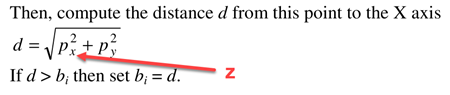Axial distance computation (typo at page 3).

One obvious drawback of M. Watkins' algorithm is that it indifferently skips feature edges. From the image below, one could easily see that the probe points are rarely coincident with the model edges. The initial distribution of slices by bins leaves little chance to capture sharp corners. That is the price of simplicity, and the trivial way to improve the result is using many more bins (e.g., I ended up with 100).

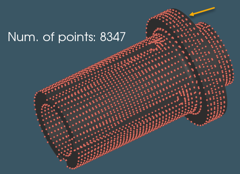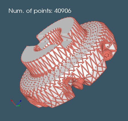
The computed intersection points.

The value stored in each bin is the radius value we are looking for. There are as many points as many slicing planes (bins) you asked the algorithm to generate.

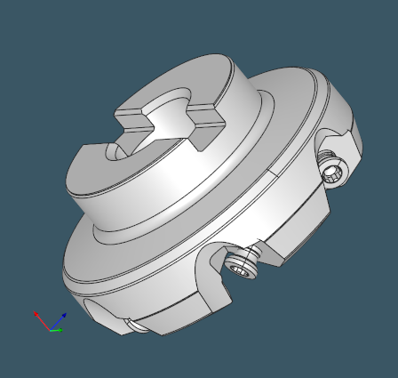Initial mill part.

The algorithm is insensitive to the quality of the input meshes. I have had hard times trying to refine meshes to make them more suitable for other algorithms, so I could definitely appreciate that. No need to think much about the aspect ratios of your triangles whatsoever.

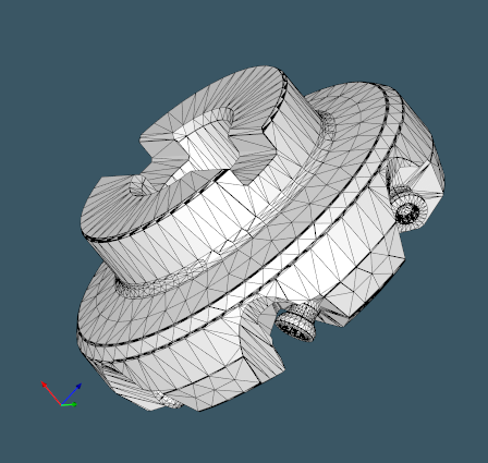The derived visualization mesh.

The process of slicing is trivial as it all comes down to intersecting mesh edges and planes. You do not even need any planes as the problem is essentially reduced to one dimension.

Intersection points on mesh edges.

Having all intersection points, it's trivial to select ones that yield the max distance at each axial bin. After connecting those points with the straight line segments using something like BRepBuilderAPI_MakePolygon, you end up with the generatrix profile.

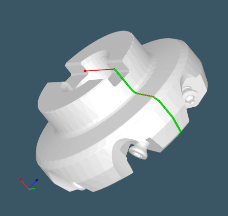Points of max distance.

It's a no-brainer then to call BRepPrimAPI_MakeRevol to build up the swept solid.

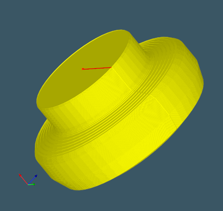The solid of revolution.

The algorithm is not ideal as it cannot stack up several slices in one bin, and that makes it incapable of capturing planar turn faces. Still, the approximation is quite good, and one might want to add small proximity offset to the profile for safe collision tests (if that's what you're looking for).

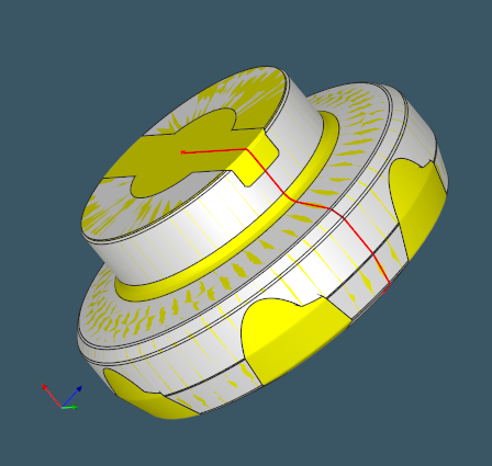The initial part and its swept volume.

To conclude, this approach is easy to implement, it's fast and reliable, and it tolerates bad meshes as the input.

Turned volume

We would normally want to compute some global properties of a swept body, e.g. its volume. The easiest way would be constructing the explicit B-rep geometry of the corresponding solid of revolution and running something like BRepGProp on it. At the same time, unless we really need to have the explicit boundaries of the swept body (e.g. for collision tests), there's no need to dive into geometric computations anymore. Given that we can represent our profile as a scalar function, it's not difficult to integrate it along the OX axis.

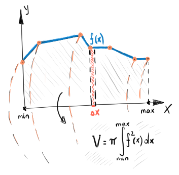To the volume computation.

One easy way to turn our profile into a function that could undergo integration is by representing it as a 1-degree spline curve. For example like this:

Handle(Geom_BSplineCurve)
  PolylineAsSpline(const std::vector<gp_XYZ>& trace,
                   const double               minKnot,
                   const double               maxKnot)
{
  TColgp_Array1OfPnt poles( 1, (int) trace.size() );
  for ( size_t k = 0; k < trace.size(); ++k )
  {
    poles( int(k + 1) ) = gp_Pnt( trace[k] );
  }
  
  const int    n    = poles.Upper() - 1;
  const int    p    = 1;
  const int    m    = n + p + 1;
  const int    k    = m + 1 - (p + 1)*2;
  const double span = (maxKnot - minKnot) / (k + 1);
  
  // Knots.
  TColStd_Array1OfReal knots(1, k + 2);
  knots(1) = minKnot;
  //
  for ( int j = 2; j <= k + 1; ++j )
  {
    knots(j) = knots(j-1) + span;
  }
  knots(k + 2) = maxKnot;
  
  // Multiplicities.
  TColStd_Array1OfInteger mults(1, k + 2);
  mults(1) = 2;
  //
  for ( int j = 2; j <= k + 1; ++j )
  {
    mults(j) = 1;
  }
  //
  mults(k + 2) = 2;
  
  return new Geom_BSplineCurve(poles, knots, mults, 1);
}

For the integration, one could use something like Gaussian quadratures. I implemented them once and it was working nicely. The only trick is to perform integration by knot spans for a better accuracy:

// Evaluate using Gaussian integration in knot intervals.
const TColStd_Array1OfReal& knots        = profileCurve->Knots();
const int                   nGaussPts    = 6;
double                      precGaussVal = 0;
for ( int k = knots.Lower(); k < knots.Upper(); ++k )
{
  const double
    intervGaussVal = core_Integral::gauss::Compute(&fx,
                                                   knots(k),
                                                   knots(k+1),
                                                   nGaussPts);
  //
  precGaussVal += intervGaussVal;
}
double SweptVolume = precGaussVal;

Here 'fx' is the function object that returns the squared radius of rotation for the given value of 'x' multiplied by Pi. As a result, we avoid using any topological primitives and derive what we need from the profile polyline.

Conclusion

The main downside of the outlined MTS algorithm is its incapability of capturing sharp corners of a model. That might be critical for applications where high accuracy is a must. On the other hand, Watkins algorithm is easy to implement and it's pretty darn fast. Even for complex models, it takes a fraction of a second. Another shiny property of the algorithm is its robustness. Since the logic is straightforward, there's almost nothing to debug and you can get to the stable version real quick.

On medium.com

Want to discuss this? Jump in to our forum.