Лучшие практики

Motivation

We are going to discuss the generalization of a Coons patch for interpolating curve networks. So, Gordon surfaces. These surfaces were introduced by W. Gordon in the late 1960s when he was working for the General Motors Research labs. It was Gordon who coined the term transfinite interpolation for the surfaces passing exactly through the curves of interest.

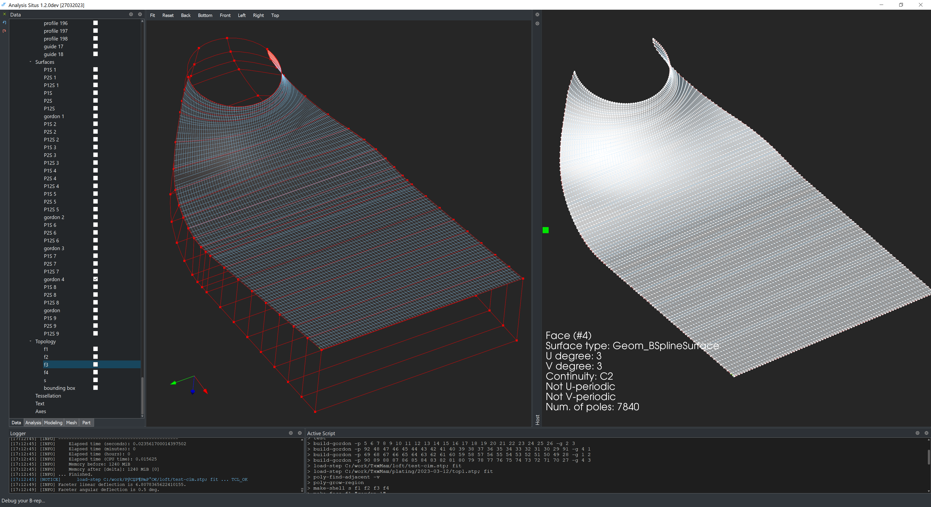Gordon surface constructed as a B-spline surface for a turbomachinery component.

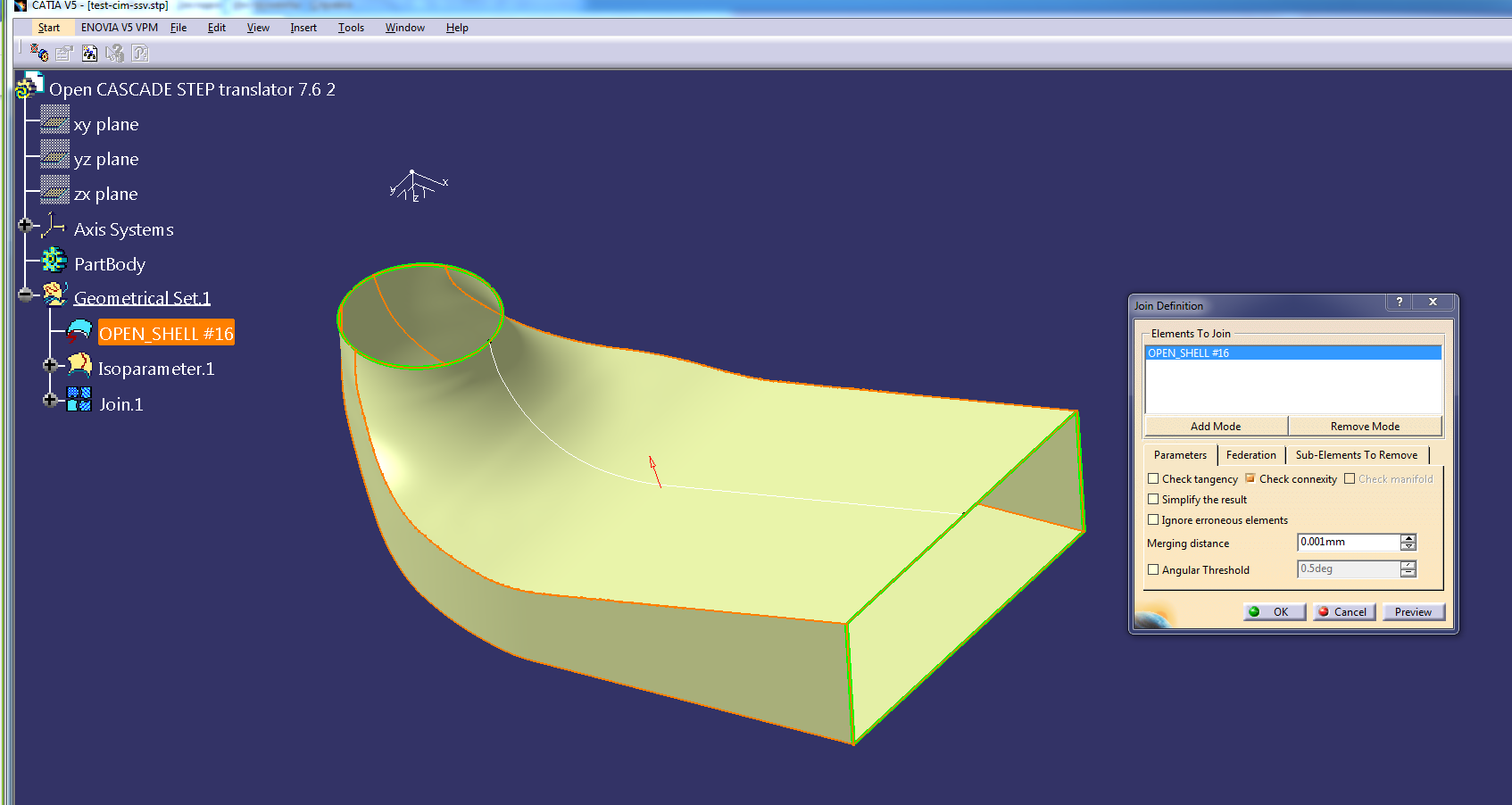Gordon surfaces constructed in Analysis Situs and exported to Catia.

For the practical perspective on this problem, you may want to check the corresponding discussion at FreeCAD forum, which is absolutely worth reading. Another source of knowledge is definitely the Curves Workbench of the same good old FreeCAD. Anticipating some criticism on why we're reinventing the wheel instead of using what FreeCAD or TiGL have to offer, here are some restrictions we have to deal with:

1. We need to have full control over the sources, which, I believe, is the only way towards real maintainability.
2. As in the beginning of any research, I'm simply not sure what's going or not going to work, and the best way to get to know this is to drop some C++ in your IDE and build the thing on your own.
3. Ultimately, we have to end up with curve and surface modeling subsystem in Analysis Situs to later bridge it with Salome for mesh generation workflows. Using FreeCAD for one thing, TiGL for another and Catia for the 3-rd is not an option and is absolutely no fun.

Formalism

Do you really want Lagrange?

A transfinite interpolation scheme consists in composing a Boolean sum (see sec. 22.8 in G. Farin's "Curves and Surfaces for CAGD" for the definition of Boolean sums) surface written as

$\begin{equation} \textbf{S} = \textbf{S}_1 + \textbf{S}_2 - \textbf{S}_{12} \label{eq:boolean-sum} \end{equation}$

Here $\textbf{S}_1$ is an interpolant to profile curves, $\textbf{S}_2$ is an interpolant to the guide curves, and $\textbf{S}_{12}$ interpolates the regular grid of points where the profile curves intersect the guide ones.

In Lagrangian form, you can write the term $\textbf{S}_1$ as

$\textbf{S}_1 = \sum_{i=0}^{m} \textbf{c}(u,v_i) L_{i}^{m}(v)$,

where $\textbf{c}(u,v_i)$ is the i-th profile curve and $L_{i}^{m}$ is the Lagrange polynomial of degree $m$ (imagine how computationally "nice" they are becoming for 20 profiles). In the same manner, we have

$\textbf{S}_2 = \sum_{j=0}^{n} \textbf{c}(u_j,v) L_{j}^{n}(u)$,

where $\textbf{c}(u_j,v)$ is the j-th guide curve. Finally, for the pointwise interpolation, we can set

$\textbf{S}_{12} = \sum_{i=0}^{m} \sum_{j=0}^{n} \textbf{c}(u_j,v_i) L_{j}^{n}(u) L_{i}^{m}(v)$,

where $\textbf{c}(u_j,v_i)$ are the curve network intersection points.

Probably the only advantage of Lagrange basis is that it is easy to verify that the Boolean sum surface $\eqref{eq:boolean-sum}$ passes through the input curve network precisely. This is enough for theoretical considerations, and that is probably why this formulation is used by G. Farin in his "Curves and Surfaces for CAGD" and also by N. Golovanov is the C3D book "Geometric modeling". On the other hand, such formulation is completely impractical for a geometric modeling system, because:

1. Lagrange polynomials expose higher and higher degrees with adding more and more curves to the network.
2. Any Lagrange-based surface is not standard (keep in mind STEP or IGES) and would require reapproximating with splines to be communicated between software packages.

There are at least two good papers that develop the concept of Gordon surfaces further for CAGD:

• [Lin F., Hewitt W.T. Expressing Coons-Gordon surfaces as nurbs // Computer-Aided Design. 1994. N 2 (26)]
• [Siggel, M., Kleinert, J., Stollenwerk, T., & Maierl, R. (2019). TiGL: An Open Source Computational Geometry Library for Parametric Aircraft Design. Mathematics in Computer Science, 13(3), 367–389]

The paper by F. Lin and W.T. Hewitt reformulates Gordon in the B-spline basis. Then, the paper by M. Siggel et al provides some useful insights on the same subject and presents their TiGL software package. Actually, TiGL is probably the ultimate solution to Gordon, so you can even stop reading here and check out TiGL for a workable implementation (I did it myself, and it was operational).

Still reading this? Then, let's discuss what it takes to express Gordon with splines.

Procedural approach with splines

Constructing a Gordon surface bottom-up with splines is really like a programming exercise and not like putting together a mathematical formula in MATLAB whatsoever. I would even say it's a bit mysterious process, because you do not deal with these "nice" (for mathematical proofs only?) Lagrange coefficients but it kinda still works if you manage to compose a Boolean sum on the procedurally defined projector operators $\textrm{P}_1$, $\textrm{P}_2$, $\textrm{P}_{12}$. On the other hand, it's much easier to make a mistake with splines compared to Lagrangian basis. You should be exceptionally delicate with the analytical props of your geometry, because otherwise your outcome surface easily goes wild and stops respecting any curve boundaries.

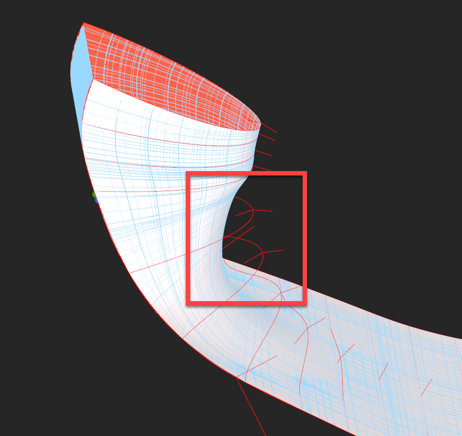Broken Gordon.

In the image above, the surface $\textbf{S}_2$ failed to catch up with the surface $\textbf{S}_{12}$ due to their different parameterization velocities. The Boolean sum $\eqref{eq:boolean-sum}$ would not work for asynchronous splines, and the final surface would get internal sinks and unpredictable shape defects. A spliny Gordon is very (very!) sensitive to the parameterizations of $\textbf{S}_1$, $\textbf{S}_2$ and $\textbf{S}_{12}$. These surfaces all have to be completely synchronous, not just "compatible" in the B-spline sense: having identical knot vectors and degrees is NOT enough. Evaluated in 3D, all knots should bring you to the same point given that the corresponding surfaces are stacked upon each other.

The surfaces $\textbf{S}_1$ (P1S) and $\textbf{S}_{12}$ (P12S) should have the same parameterization velocity: this can be seen by knot isolines joining each other.

Without being able to analyze knot distribution over the surfaces, you might end up in desperate debugging your Gordon procedure for surfaces that might look visually perfect but remain analytically wrong.

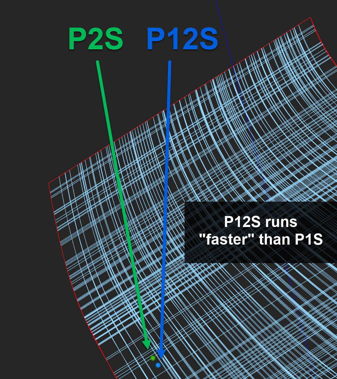This picture demonstrates how the parameterization velocity of the Boolean sum surfaces can be different. Here, the surface P12S constructed by interpolating intersection points runs faster than the surface P1S in the corresponding curvilinear direction. Those surfaces are not acceptable for Gordon.

So what would be the correct way of constructing a Gordon surface for the given network of curves? Let's have a look at a somewhat simple example.

Curve network: guides $\textbf{g}_i$ and profiles $\textbf{p}_j$.

Given a set of guide curves $\textbf{g}_i$ and profile curves $\textbf{p}_j$, we seek to construct the Gordon surface $\textbf{S}(u,v)$ having the transfinite interpolation property over those curves. The procedure starts by extracting all intersection points $\textbf{Q}_{ij}$ for the curves in the initial network. The purpose of extracting those points is twofold:

1. We need to extract the Cartesian coordinates of those points $(x,y,z) = \textbf{Q}_{ij}$. That is because the projector $\textrm{P}_{12}$ is going to interpolate them to build the surface $\textbf{S}_{12}$. We refer to this stage as "curve intersection".
2. We need to compute the parameters of those points as $t_g = \left[\textbf{Q} \to \textbf{g}\right]$ and $t_p = \left[\textbf{Q} \to \textbf{p}\right]$ on the corresponding curves (we denote point inversion operator as $\to$). Those parameters should later be passed into the skinning and interpolation projectors $\textrm{P}_{1}$, $\textrm{P}_{2}$ and $\textrm{P}_{12}$ in order to obtain the exactly synchronous surfaces. We refer to this stage as "point parameterization".

Intersection points between guide and profile curves.

But before the curves are intersected, it is necessary to turn them into a compatible form.

Making curves compatible

Compatibility of curves means several things:

1. All curves should be represented as B-spline curves.
2. The curves should have the same degrees. If not, their degrees should be elevated to the max degree among the curve set.
3. The curves should have the same direction of parameterization.
4. The guide and profile curves should have the same origin point.

Incompatible curves due to inconsistent flow directions.

Curves should be properly sorted.

Inconsistent origins of profiles w.r.t. guides.

Compute intersection points

Curve intersection is done by the algorithm we borrowed from TiGL (thanks!).

Since we are dealing with a grid of intersection points, their $u$ and $v$ parameters can be stored in two matrices (one for profile curves and another for guides).

Intersection points to compute.

For the curve network presented above, those matrices might look something as follows:

profile 1 | 0 0.494674 1
----------+--------------
profile 2 | 0 0.48623  1
----------+--------------
profile 3 | 0 0.576487 1
----------+--------------

guide 1  | guide 2 | guide 3
---------+---------+----------
0        | 0       | 0
0.539844 | 0.48561 | 0.498426
1        | 1       | 1

Any of those tables can be used to evaluate the 3D coordinates of the intersection points among curves and pass them to the projector $\textrm{P}_{12}$.

Middle intersection point for a curve network.

We could have evaluated any of the two intersecting curves and obtain the same 3D coordinates.

Different $(u,v)$ parameters correspond to the same point.

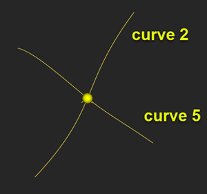
Intersection points for a curve network.

There is one problem with these intersection parameters that is not obvious at all. Even if the initial profile and guide curves were reapproximated on the same knot vector and parameter values (i.e., they are skinning-ready), they are not "synchronous enough" for Gordon. To see why, it is enough to trace how an intersection point parameters evolve from profile to profile.

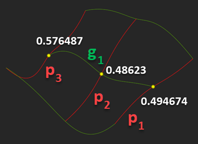Different parameters of an isoline.

If we require that the curve $\textbf{g}_1$ (see image above) is becoming an isoparametric curve of the final surface (and this is due to the definition of a Gordon surface), then it should travel over the corresponding intersection points all having the same parameter value across the profile curves $\textbf{p}_j$, where $j=1,2,3$.

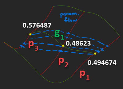Bad parameter flow of otherwise perfectly synced curves.

The latter fact basically means that the input profile and guide curves should not be just skinning-wise synchronous. They should be pointwise synchronous to avoid any parameter flow twists not respecting the intersection points between the curves. In practice, this would mean that the algorithm has to:

1. First, compute the intersection points between curves.
2. Reapproximate curves all together while making sure they are synced by the passage parameters at the computed intersection points.

One addition here is that to facilitate the first stage (intersection points computations) it might be necessary to reapproximate curves just to make them better suited for the intersection algorithm. As a result, it might be necessary to reapproximate the constraint curves twice, which is the computational reality you have to face, like it or not.

UI

Gordon surfacing requires that the profile and guide curves are specifically prepared beforehand, namely:

1. Curves should be maximized, i.e., they should not accommodate any smaller segments. For example, a guide curve should travel all along profile curves without any intermediate breakpoints (vertices). If that's not the case, the corresponding edges can be concatenated using the context-menu function of Analysis Situs (specifically added for Gordon preparation).
2. Curves should geometrically intersect each other, although those intersection points are not explicitly available right away.

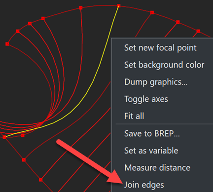Concatenation of edges.

To proceed with Gordon surfacing, you should load a wireframe model to Analysis Situs (as STEP, IGES or BREP) and run the "Build Gordon surface..." action from the context menu of the Part Viewer. This action will bring you to the surface definition dialog as shown in the following image:

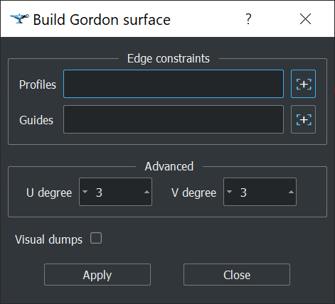Gordon surface definition dialog.

Using the "[+]" button, invoke the interactive selector of profiles and guides. Use <SHIFT> button for multiple selection of edges (make sure that edge selection mode is activated).

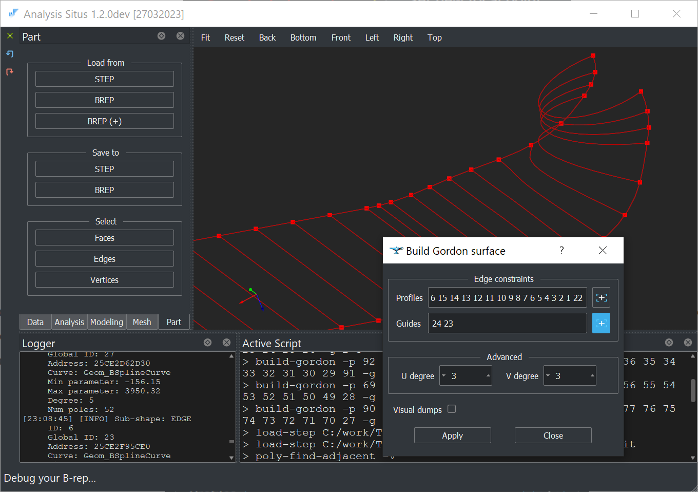Finished selection of profiles and guides.

Click "Apply" button to build the final surface.

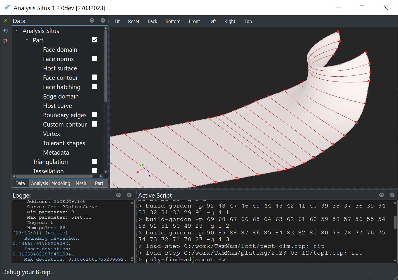Final Gordon surface.

Want to discuss this? Jump in to our forum.