Архивы

Flattening cylinders

Read Part 1 to familiarize with the principle of sheet metal unfolding.

Intro

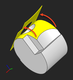
One of the essential ingredients of the unfolding algorithm is flattening bend faces. This article explains how to unwrap cylinders (the canonical host surfaces of bends) while preserving all their contours, including carved edges and holes. The unfolding is done without deformations, i.e., not taking K-factor into account. The application of material props is left for future investigation. As usual, we start by preparing a test case in Analysis Situs:

Preparing a test case for unwrapping a non-trivially trimmed cylindrical face.

The cylindrical top face of the obtained CAD part is something we would like to unfold. All carving edges, including the inner loop should be preserved in the flat shape. Here is the parametric portrait of that face:

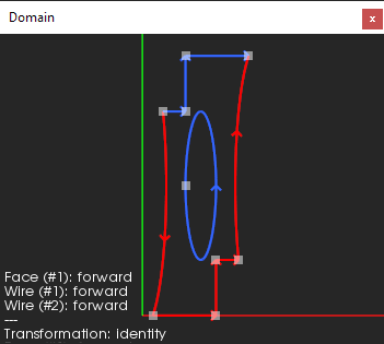The parametric domain of the carved cylindrical face to unfold.

Notice that we cannot merely take the two-dimensional portrait of the face as it is fundamentally distorted. That's not a surprise as the curvilinear axes of a cylindrical face represent its angle (U axis) and height (V axis). While the height (V axis) preserves the modeling space metric, we still have to do something with the angular dimension (U axis).

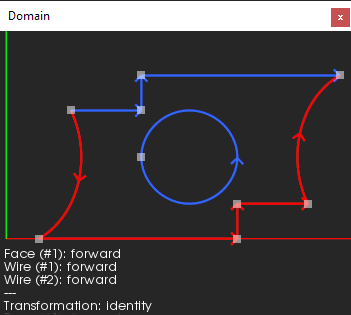The parametric domain of the unfolded face we'd like to achieve.

While it is generally desirable to get the inner loop as a circle in two-dimensions, such a requirement is somewhat harder to satisfy. Let's set the following guiding rules for the unfolding algorithm instead:

1. If a two-dimensional curve of the parametric domain is parallel to the U or V axis, its image in the flat pattern is a three-dimensional straight line.
2. In other cases, let's just approximate the three-dimensional curve with a B-spline curve (B-curve).

If we'd ever want to get analytical images of circles in the flat pattern, we'd need to add some sort of analytical recognition as a post-processing stage. Even though such an extension might be of the high demand for obtaining accurate drawings, let's omit this for now.

Idea of the algorithm

There should be a reference plane where the flat pattern is supposed to reside. The choice of the reference plane is left to the main unfolding algorithm, so here we are not bothered to select it. Let's just take the XOY plane as a reference. Our flattening algorithm takes the input cylindrical face and constructs the resulting face without boundaries as the following code snippet shows:

// m_resFace is the result face.
// m_refPlane is the reference plane.
BRep_Builder().MakeFace( m_resFace,
                         new Geom_Plane(m_refPlane),
                         Precision::Confusion() );

The very idea of the algorithm is to reconstruct boundaries. That's pretty obvious as the reference plane being a host surface for our resulting face is infinite, so we have to trim it properly. The most interesting piece of logic here is the unwrapping of edges. Unwrapping an edge is a two-ingredient problem:

1. The topological formation of an edge (simple one).
2. The geometric formation of an edge (harder problem).

The geometric formation of an edge employs constructing its extremities (three-dimensional points), a three-dimensional curve (as the primary edge representation), and a parametric curve (pcurve). In OpenCascade, the edges residing on the planar faces are not obliged to have parametric curves, so we're going to take advantage of that fact and save some efforts. The missing pcurves for the planar faces are constructed on the fly, whenever the calling code asks for them.

The reconstruction of curves can be done using the approximation framework of OpenCascade: AdvApprox_ApproxAFunction by Xavier Benveniste (currently a technology director in R&D of SolidWorks). To use it, one has to derive a subclass from the basic AdvApprox_EvaluatorFunction class shipped with OpenCascade. The function to reapproximate is $f : R \to R^2$. Here $f = \textbf{c}(t)$ and $\textbf{c}(\cdot)$ is the pcurve we want to unwrap.

//! A function to be approximated by AdvApprox_ApproxAFunction.
class Evaluator : public AdvApprox_EvaluatorFunction
{
public:
  
  //! Ctor with initialization.
  Evaluator(const Handle(Geom2d_Curve)&         c2d,
            const Handle(GeomAdaptor_HSurface)& surf)
  : m_c2d(c2d), m_surf(surf)
  {
    m_fR = m_surf->Cylinder().Radius();
  }
  
public:
  
  //! Evaluates the function to reapproximate.
  virtual void Evaluate(int*,
                        double[2],
                        double*    t,
                        int*       DerivativeRequest,
                        double*    Result,
                        int*       ReturnCode)
  {
    gp_Pnt2d P;
    gp_Vec2d V;
    
    if ( *DerivativeRequest == 0 )
    {
      m_c2d->D0(*t, P);
      
      Result[0] = m_fR * P.X();
      Result[1] = P.Y();
    }
    else if ( *DerivativeRequest == 1 )
    {
      m_c2d->D1(*t, P, V);
      
      Result[0] = m_fR * V.X();
      Result[1] = V.Y();
    }
    
    ReturnCode[0] = 0;
  }
  
private:
  
  Handle(Geom2d_Curve)         m_c2d;
  Handle(GeomAdaptor_HSurface) m_surf;
  double                       m_fR;
  
};

It is the job of AdvApprox_ApproxAFunction to supply our custom evaluator with the $t$ parameter. It may also ask for the function derivative using the DerivativeRequest argument. Notice that in our custom evaluator we implement special care for scaling the resulting coordinates in U direction. The scaling rule is $R \cdot c_x(t)$ or $R \cdot c'_x(t)$ where $R$ is the cylinder radius and $c_x$ is the component of vector-valued function $\textbf{c}$ in its angular direction. The evaluated point (after scaling) is returned to the Result variable which is the two-dimensional array. AdvApprox_ApproxAFunction knows what to do next to build up a couple of new polynomial functions (for each coordinate separately). To supply our evaluator to the AdvApprox_ApproxAFunction tool, one can use the following code:

// Prepare custom function for approximation.
Evaluator Eval(c2d, surf);
Handle(TColStd_HArray1OfReal) tol1d, tol2d, tol3d;
tol1d = new TColStd_HArray1OfReal(1, 2);
tol1d->SetValue( 1, surf->UResolution(tol) );
tol1d->SetValue( 2, surf->VResolution(tol) );
  
// Approximate.
AdvApprox_ApproxAFunction approx(2, 0, 0, tol1d, tol2d, tol3d, f, l,
                                 GeomAbs_C1, 12, 100,
                                 Eval);

The only missing puzzle piece here is how to construct a B-curve out of the approximation result. The thing is that AdvApprox_ApproxAFunction does not perform such a conversion by itself. It only returns two independent functions for each coordinate. To fill the gap, the supplementary GeomLib_MakeCurvefromApprox utility should be used:

GeomLib_MakeCurvefromApprox buildBCurve(approx);
Handle(Geom2d_BSplineCurve) result = buildBCurve.Curve2dFromTwo1d(1, 2);

What this utility does is pretty straightforward. It takes all necessary props from the approximator and constructs a well-formed B-curve without applying any extra logic down the road. Here is the simplified code excerpt from the OpenCascade sources:

Handle(Geom2d_BSplineCurve)
  GeomLib_MakeCurvefromApprox::Curve2dFromTwo1d(const Standard_Integer Index1d,
                                                const Standard_Integer Index2d) const 
{
  TColgp_Array1OfPnt2d    Poles    ( 1, myApprox.NbPoles() );
  TColStd_Array1OfReal    Poles1d1 ( 1, myApprox.NbPoles() );
  TColStd_Array1OfReal    Poles1d2 ( 1, myApprox.NbPoles() );
  TColStd_Array1OfReal    Knots    ( 1, myApprox.NbKnots() );
  TColStd_Array1OfInteger Mults    ( 1, myApprox.NbKnots() );
  
  myApprox.Poles1d(Index2d, Poles1d2);
  myApprox.Poles1d(Index1d, Poles1d1);
  
  Knots = myApprox.Knots()->Array1();
  Mults = myApprox.Multiplicities()->Array1();
  
  for ( Standard_Integer i = 1; i <= myApprox.NbPoles(); i++) {
    Poles(i).SetCoord(Poles1d1.Value(i),Poles1d2.Value(i));
  }
  
  Handle(Geom2d_BSplineCurve) C =
    new Geom2d_BSplineCurve( Poles, Knots, Mults, myApprox.Degree() );
  
  return C;
}

You might have noticed that myApprox (the instance of AdvApprox_ApproxAFunction) can provide all necessary basis props, so it's not B-spline agnostic.

The unfolded top face.

The unwrapped face resides in the reference plane. To give it a proper position in the final flat pattern, it is necessary to supplement the flat face with a movement transformation.

Now that we know how to unwrap a cylindrical face precisely, it is time to consider the technological side of the issue. In reality, bends are never unfolded without deformation. There is always some thickness that contributes to the distortion of the material, so unfolding is not a purely geometric problem. We will cover this topic in the upcoming blog post.

You can also read this article on Medium.com.

Want to discuss this? Jump in to our forum.