Архивы

"If you can't have fun, there's no sense in doing it." One famous guy.

A typical "hello world" application with OpenCascade is building up a cube. However, such a model is a way too simplistic for what we're going to discuss today.

This week I faced a need to investigate the accuracy issue in one of our voxelization algorithms. Testing such sort of things on the parallelepiped-like domains is nonsense as the involved surfaces are all planar. Of course, if the voxelization algorithm employs octree subdivision, you may rotate your cube to get a denser grid over the faces. Such a "trick," however, does not look sufficient for a fair test. All voxelization tools start from a tessellated representation of a geometry. A cubical shape is captured by twelve triangles only, no matter how you set up the transformation matrix. Therefore, to dive into real accuracy problems on voxelization, you'd better take a more sophisticated example. So imagine the following testing scenario:

1. A curved model is tessellated. Here we get the first approximation error.
2. A voxelization representing this model as a signed distance field is constructed. Here we might get additional imprecision as we switch from the Lagrangian boundary representation to a space grid.
3. The distance field is converted back to mesh using one of the polygonizing algorithms, such as marching cubes. Here, again, some error might occur due to the polygonization.

You may wonder if such a workflow makes any sense. Well, here is how it goes. We start from a mesh representation, then pass it through the voxelization algorithm, then get back the polygonized model. Why is this? The answer resides in the quality of both meshes (the input and the output ones). Although the input and output triangulations are geometrically similar, we are guaranteed to obtain a watertight mesh as a result, even for a "dirty" input. Here, the voxelizer serves as a filter to eliminate any topological flaws. To test such a workflow, we need some curved geometry that encloses a finite volume in modeling space. Let's apply a bit of distortion to a simple cube case, and go for a sort of a wavy cube instead.

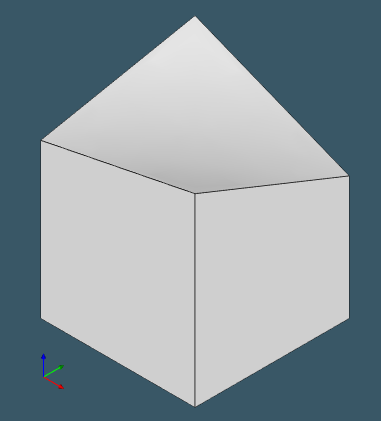A wavy cube.

So we go and create our shape patch-by-patch. One option here is to use bilinear Coons surfaces for representing each face. The following script does this in a very straightforward way. Notice that we interpolate curves more than necessary, and in a smarter procedure, we would, of course, do only 12 approximations instead of 24 applied below. However, such duplication allows us to keep the code a bit more structured.

> clear
> make-point p1 0 0 0
> make-point p2 1 0 0
> make-point p3 1 1 0
> make-point p4 0 1 0
> make-point p5 0 0 1
> make-point p6 1 0 1.2
> make-point p7 1 1 0.8
> make-point p8 0 1 1.2
  
> interpolate-points c1 -points p1 p2 -degree 1
> interpolate-points c2 -points p4 p3 -degree 1
> interpolate-points b1 -points p1 p4 -degree 1
> interpolate-points b2 -points p2 p3 -degree 1
> build-coons-linear s0 c1 c2 b1 b2
  
> interpolate-points c1 -points p5 p6 -degree 1
> interpolate-points c2 -points p8 p7 -degree 1
> interpolate-points b1 -points p5 p8 -degree 1
> interpolate-points b2 -points p6 p7 -degree 1
> build-coons-linear s1 c1 c2 b1 b2
  
> interpolate-points c1 -points p1 p5 -degree 1
> interpolate-points c2 -points p2 p6 -degree 1
> interpolate-points b1 -points p1 p2 -degree 1
> interpolate-points b2 -points p5 p6 -degree 1
> build-coons-linear s2 c1 c2 b1 b2
  
> interpolate-points c1 -points p2 p3 -degree 1
> interpolate-points c2 -points p6 p7 -degree 1
> interpolate-points b1 -points p2 p6 -degree 1
> interpolate-points b2 -points p3 p7 -degree 1
> build-coons-linear s3 c1 c2 b1 b2
  
> interpolate-points c1 -points p1 p5 -degree 1
> interpolate-points c2 -points p4 p8 -degree 1
> interpolate-points b1 -points p1 p4 -degree 1
> interpolate-points b2 -points p5 p8 -degree 1
> build-coons-linear s4 c1 c2 b1 b2
  
> interpolate-points c1 -points p3 p4 -degree 1
> interpolate-points c2 -points p7 p8 -degree 1
> interpolate-points b1 -points p3 p7 -degree 1
> interpolate-points b2 -points p4 p8 -degree 1
> build-coons-linear s5 c1 c2 b1 b2
  
> make-face f0 s0
> make-face f1 s1
> make-face f2 s2
> make-face f3 s3
> make-face f4 s4
> make-face f5 s5
  
> make-shell shell f0 f1 f2 f3 f4 f5
> make-solid solid shell
> set-as-part solid
> sew
> invert-shells
> donly

A wavy cube in Analysis Situs.

Bicubic B-surfaces represent all faces of the final solid. Another lovely property of the resulting shape is that it possesses just a perfect boundary proximity. These very tight tolerances are obtained thanks to utilizing a curve network and avoiding building up any trimmed patches.

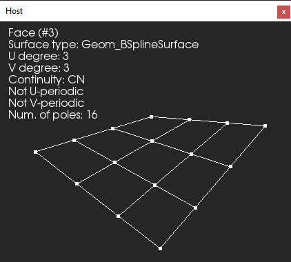A host surface of a top face.

You may notice that in the course of construction, we did not pay attention to our patches' geometric orientations. By construction, some of the Coons surfaces happen to be oriented inside the enclosed material. It is not necessary to fix such an issue, though, as the sewing operator handles it later. In this scenario, however, the final solid happens to be inverted, so we have to reverse it to obtain the result that we want.

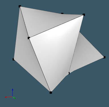A tricky "wavy cube." Still perfectly watertight.

You may obtain more tricky shapes of a wavy cube by playing with the coordinates of its vertices.

On Medium.com